In this post I want to cover some interesting things about step response and I hope to clarify via examples what the step response is and how it can be used to specify the design for closed-loop control systems, to do that I will use program laguage for Octave. So, to answer the question “What is the step response?” we can simply say that it is how a system responds to a step input, it means that we can input a unit step function into a system and we can measure how the systems responds to that.
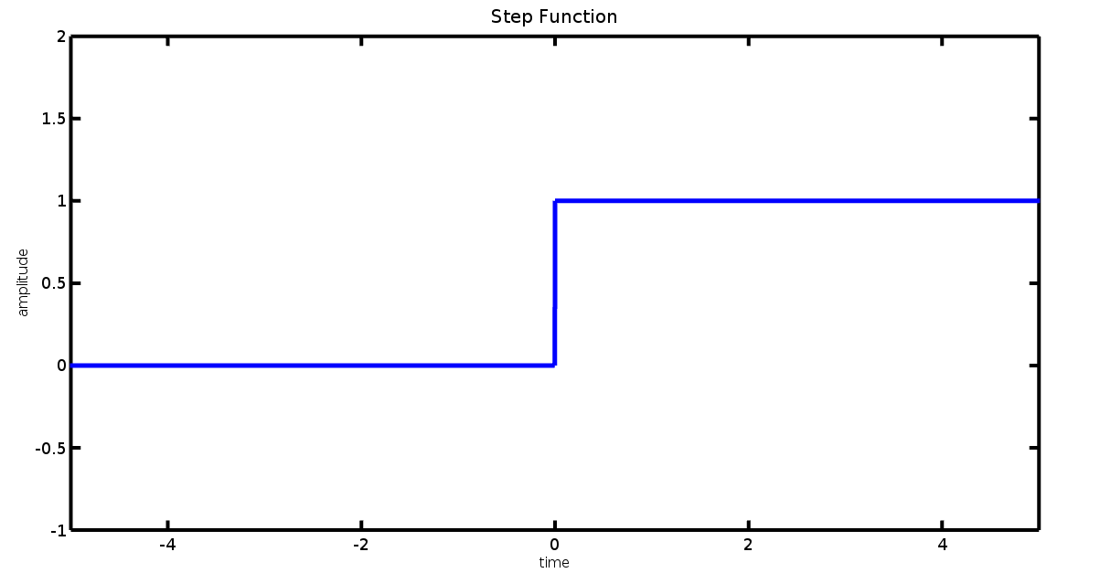
But I know, maybe you are asking yourself “And what about the step function?”, it is simple also, the step function is a transition from one state to another in a very very small time, instantly.
clear all                   # clear all variable
clc                         # clear screen

t=-10:0.001:10;             # time declaration
y=heaviside(t);             # step function

plot(t,y, "linewidth",5);   # plot
axis([-5 5 -1 2]);          # axis delimitation

###############################################
# Plot Configs                                #
###############################################
title("Step Function","fontsize", 20);
xlabel("time","fontsize", 16);
ylabel("amplitude","fontsize", 16);
set(gca,"linewidth", 4,"fontsize", 18);
In general, for a closed-loop system, to design a system we need to take care about four main parameters that could be aswered over the following questions:
- What is the time to achieve the final amplitude desired (Rise Time)?
- Is there overshoot?
- What is the time to achieve the response stability?
- What is the difference betwen the system amplitude and the amplitude desired (Tracked Reference)?
Step Response For Different Systems
Is very important to note that each system has a peculiar response when a step response is applied, below you can see the response for some systems.
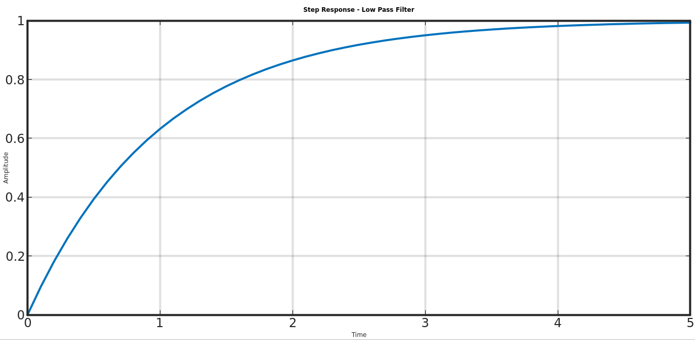
Low Pass Filter (First Order)
clear all;
clf;
s = tf('s');
g = 1/(s+1); # Low pass filter
[y,t] = step(g);
plot(t, squeeze(y), 'LineWidth',4);
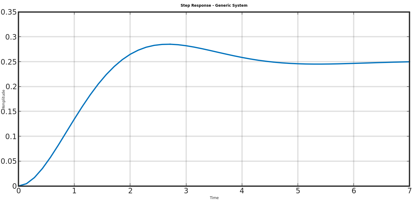
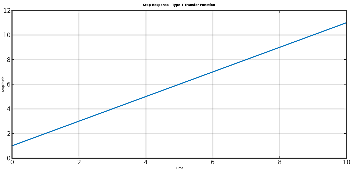
Type 1 Transfer Function
clear all;
clf;
s = tf('s');
g = 1/s*(s+1); # Type 1 transfer function
[y,t] = step(g);
plot(t, squeeze(y), 'LineWidth',4);
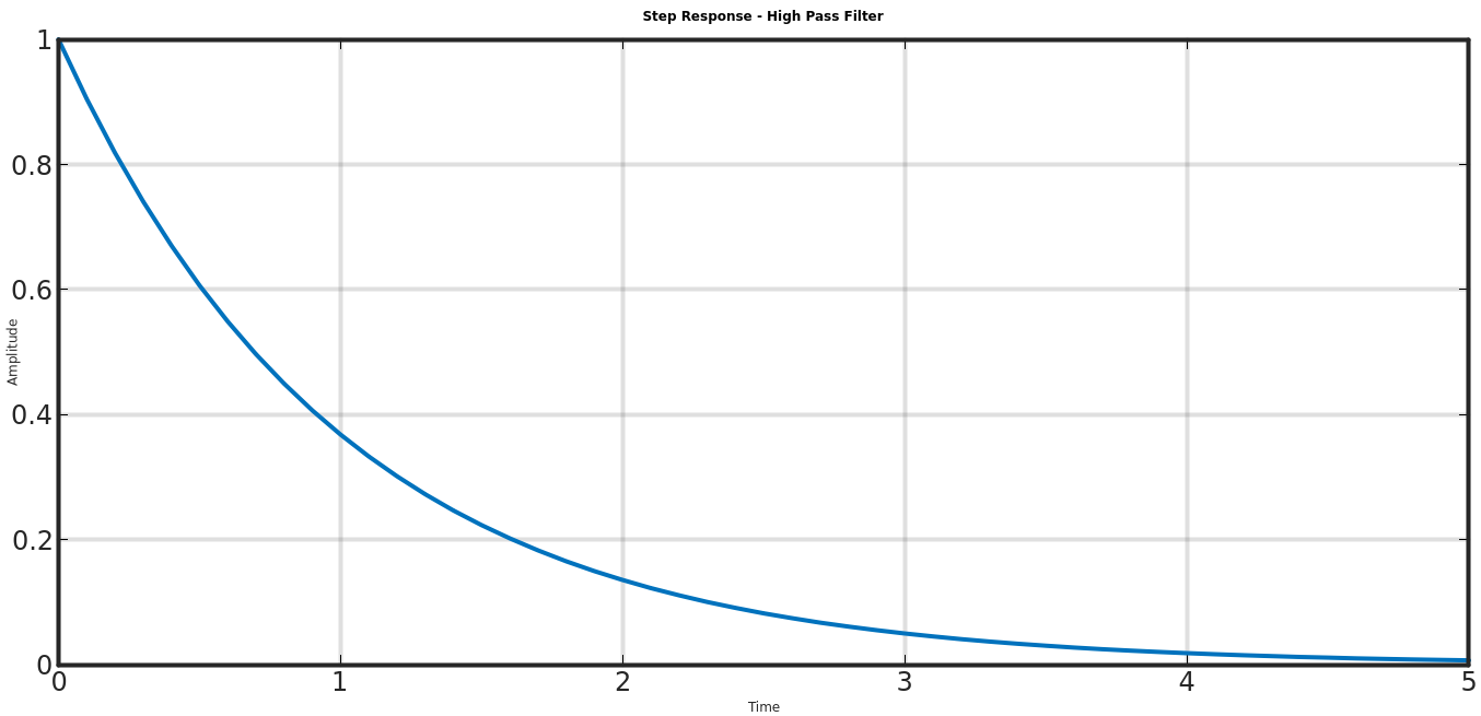
High Pass Filter
clear all;
clf;
s = tf('s');
g = s/(s+1); # High pass filter
[y,t] = step(g);
plot(t, squeeze(y), 'LineWidth',4);